Regression

The road ahead: machine learning

Five students, one question

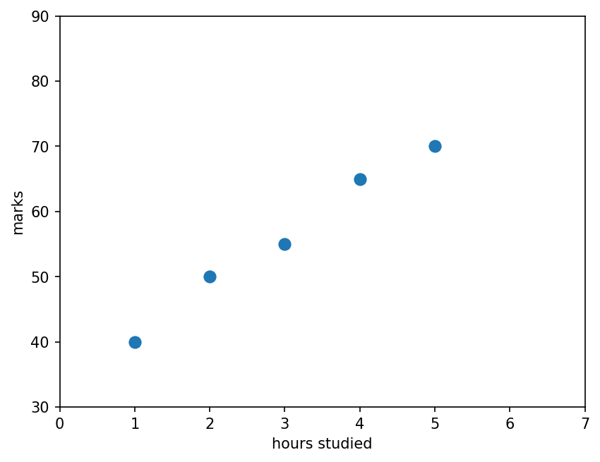
Invented data: hours studied per week and exam marks. What mark would we expect for 6 hours?

Codecopy

import matplotlib.pyplot as plt
hours = [1, 2, 3, 4, 5]
marks = [40, 50, 55, 65, 70]
plt.scatter(hours, marks, s=60)
plt.xlabel("hours studied")
plt.ylabel("marks")
plt.xlim(0, 7)
plt.ylim(30, 90)
plt.show()

Anatomy of a straight line

slope = 7.5
intercept = 33.5
h = 6
predicted = slope * h + intercept
print(predicted)

78.5

By hand: how wrong is a guessed line?

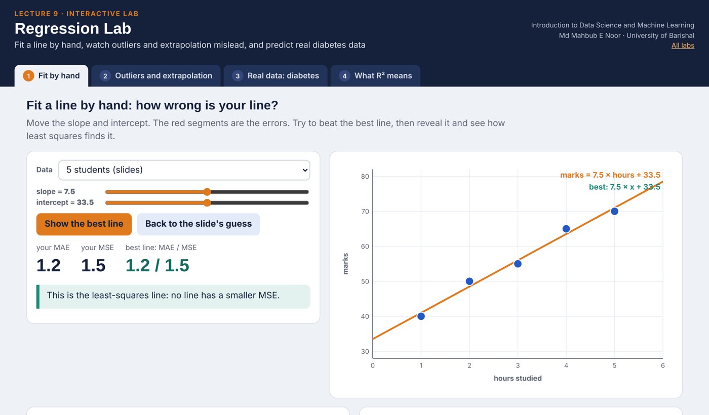
Try the line marks = 8 × hours + 30. Error = actual - predicted. MAE = average of the error sizes.

# guessed line:
#   8 * hours + 30
# MAE = (2+4+1+3+0) / 5
#     = 2.0 marks

By hand: the best line (least squares)

slope = sum of (h - mean h)(m - mean m) / sum of (h - mean h)². Means: hours 3, marks 56.

# slope = 75 / 10 = 7.5
# intercept = 56 - 7.5 * 3
#           = 33.5
# best line:
#   marks = 7.5 * hours + 33.5

The same line with scikit-learn

from sklearn.linear_model import LinearRegression
X = [[1], [2], [3], [4], [5]]
y = [40, 50, 55, 65, 70]
model = LinearRegression()
model.fit(X, y)
print(model.coef_, model.intercept_)
print(model.predict([[6]]))

[7.5] 33.5
[78.5]

Draw the fitted line

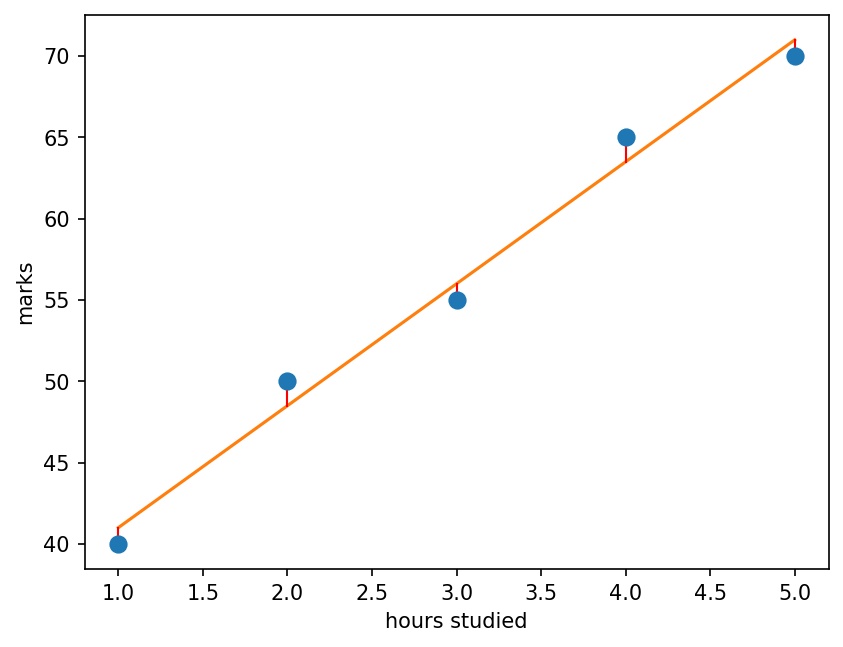
The line passes as close as possible to all points at once. The red segments are the errors it tries to keep small.

Codecopy

pred = model.predict(X)
plt.scatter(hours, marks, s=60, zorder=3)
plt.plot(hours, pred, color="tab:orange")
for h, m, p in zip(hours, marks, pred):
    plt.plot([h, h], [m, p], color="red", lw=1)
plt.xlabel("hours studied")
plt.ylabel("marks")
plt.show()

Watch it: searching for the best line

Real data: diabetes progression

from sklearn.datasets import load_diabetes
from sklearn.model_selection import train_test_split
from sklearn.metrics import mean_absolute_error
data = load_diabetes(as_frame=True)
X = data.data[["bmi"]]
y = data.target
X_tr, X_te, y_tr, y_te = train_test_split(
    X, y, test_size=0.25, random_state=0)
model = LinearRegression().fit(X_tr, y_tr)
pred = model.predict(X_te)
print(round(mean_absolute_error(y_te, pred), 1))

53.3

See why: one feature, lots of noise

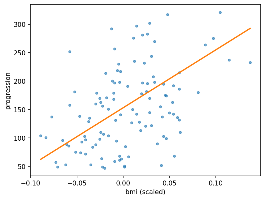
The trend is real, but patients with the same bmi differ a lot. A line can only capture the average trend.

Codecopy

plt.scatter(X_te["bmi"], y_te, s=12, alpha=0.6)
xs = X_te.sort_values("bmi")
plt.plot(xs["bmi"], model.predict(xs),
         color="tab:orange", lw=2)
plt.xlabel("bmi (scaled)")
plt.ylabel("progression")
plt.show()

All 10 features, and two more ways to score

from sklearn.metrics import r2_score
for cols in [["bmi"], list(data.data.columns)]:
    X = data.data[cols]
    X_tr, X_te, y_tr, y_te = train_test_split(
        X, y, test_size=0.25, random_state=0)
    m = LinearRegression().fit(X_tr, y_tr)
    p = m.predict(X_te)
    print(len(cols), "features: MAE",
          round(mean_absolute_error(y_te, p), 1),
          "R2", round(r2_score(y_te, p), 2))

1 features: MAE 53.3 R2 0.16
10 features: MAE 45.1 R2 0.36

What if someone studies 20 hours?

X = [[1], [2], [3], [4], [5]]
y = [40, 50, 55, 65, 70]
small = LinearRegression().fit(X, y)
print(small.predict([[20]]))

Answer: What if someone studies 20 hours?

X = [[1], [2], [3], [4], [5]]
y = [40, 50, 55, 65, 70]
small = LinearRegression().fit(X, y)
print(small.predict([[20]]))

[183.5]

Common regression mistakes

Read the last line of an error first. It names the problem.

LinearRegression().fit([1, 2, 3], [4, 5, 6])

ValueError: Expected 2D array, got 1D array instead:

LinearRegression().fit([[1], [2]], [4, 5, 6])

ValueError: Found input variables with inconsistent numbers of samples: [2, 3]

LinearRegression().predict([[6]])

NotFittedError: This LinearRegression instance is not fitted yet. Call 'fit' with appropriate arguments before using this estimator.

Today's toolkit

Homework 9

Due before Lecture 10 · [date]